I’ve used the word “catastrophic” too much these days, but like, I took my hormones to my parents, only to find out that the safe deposit I had booked cancelled on me. Now I have a ticking time bomb in my backpack.

Amazon delayed my delivered so it came after I left for my parents. By the time I will be back, the return period will have been expired.

Ali express decided to send my swimsuit to my address and not my parents. I don’t have a body of water where I live :)

How do I motivate myself to start cardio so I can loose weight?

Does my brain have a switch that i need to press?

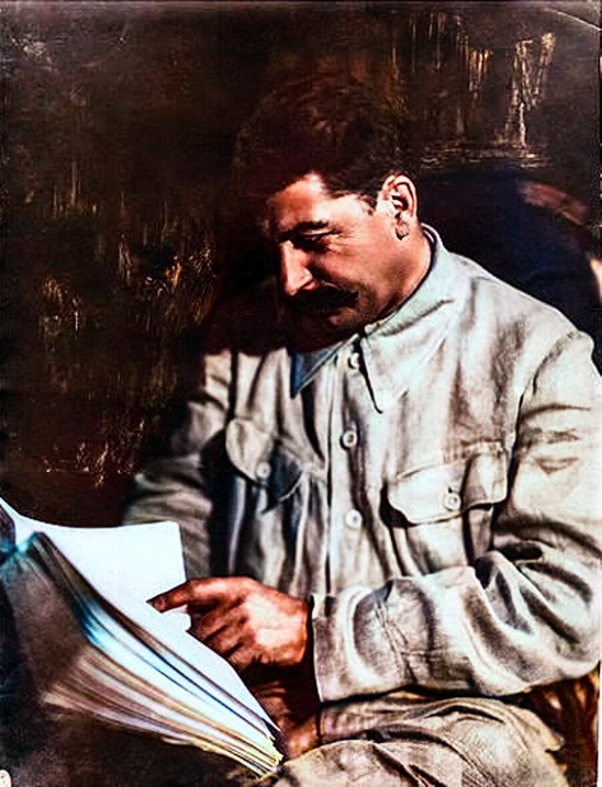
Dame Meg Hillier, who chairs the Treasury select committee and was a originally a key rebel, said “divided parties don’t hold power” and that claimed that if Labour members want to see their values played out in this country “we need to vote for this today”.

We need unity and power so we can ram through more ghoulshit policies.

I’m not kidding when I say this, kill these people.

Don’t really have many comments, but the book gets more compelling the more I read. I really like the framing of language here. Our actions, dressing, linguistic conventions aren’t simply neutral, and communicate various assumptions and notions within. That’s why it’s important to examine the language we use. Cisnormative language isn’t enough to express ourselves, which is why things like neopronouns are needed.

I tried to link all this theory with Marxism in general, because I thought it would be useful, but it doesn’t really feel like it fits. Not even into dialectics. Language might be a sort of blind spot for Marxism, despite being really important to how human societies develop.

According to the other thread, making erotica is legal but profiting off it is not. That’s the explanation. It’s still harsh though imo.

58% of Americans – 197 million people – need to be liquidated

Imagine if this was taken out of context

The above is an expression of my pain and suffering from having drunk a full glass of black coffee at 11 PM.

Forgive the lack of proper structure, I was a C student in English class.

Coffee coffee

Black coffee, Brown coffee

Make rumbly in my tummy

Make my head feel funny

Coffee coffee

A cup of no good coffee

Not sweet like toffee

Not creamy Not dreamy

Coffee coffee

taken at 23*

I feel like puking

*hour of the day, 11 PM

The Chinese statement here doesn’t even seem to understand that, thinking instead that their external regulations are PART of the market itself and that the market forces of competition are not (the opposite of reality).

This is largely a matter of semantics and it is kind of pointless to keep arguing semantics on translated text.

No, the market mechanism are working exactly as everyone knows they will by lowering the rate of profit via competition.

The market mechanisms do not directly determine the rate of profit. They only regulate the rate of profit around the value predicted by the labor theory of value (attractor point 1), which in turn is determined by the technological composition of the economy. The other attraction point of profit rates is when they are equal across sectors.

The market mechanisms are supposed to regulate the rate of profit near the 2 attraction points in marxist theory. In bourgeois economics, the attractor point of the labor theory of value is ignored.

So in a literal sense, regardless of the theory being used, it most certainly is possible for market mechanisms to stop functioning correctly, just as it is possible for a drawer to get jammed or for a car to break down.

The falling rate of profit in marxist theory does not come from competition (marx predicts decreasing competition as capitalism goes on, because of the formation of monopolies). It comes from marx’s prediction that capitalist economies become more capital intensive over time.

They just don’t like the outcome of the market system, so they want the government to step in to subsidize the corporate rate of profit

The rest of the statement literally calls for a re-evaluation of government subsidies and tax breaks, saying that they encourage a race to the bottom. Both quotes below are from the article.

as well as local officials who made misguided efforts to woo investment through unsustainable tax breaks and subsidies.

Neijuan directly affects wage levels, government tax revenues, investment confidence and the whole economy,” it said.

Increased prices of industrial goods can lead to higher government revenues and wages in China because of their status as an exporter. It means more overall revenue from sales to the west. On the other hand, low prices allow for the western economies to leech off Chinese production. In material terms, higher prices in Chinese industries means less goods are sent to the west, and thereby more goods available for consumption domestically.

They basically are so high on pro-market ideology they are unable to correctly describe the failing of the market

This is a rather large leap of logic taken from a statement that literally calls for government intervention into the market.

How is “excess competition” distorting the market mechanisms? It IS the market mechanisms. External controls to curb this would be the actual distortion of market forces.

Government regulations “distort” market mechanisms if you think that “pure” market mechanisms are those that are fully anarchic in nature.

If you approach things from a keynesian ideology (which is fairly popular in China), then market mechanisms exist to balance supply and demand, while providing incentive for innovation by firms.

In this case then, yes, the market mechanisms are not working properly. So you fix them using government intervention.

You should remember, in keynesian theory, the government and markets are supposed to support each other.

Catastrophic news. The Mao Mao cosplay I ordered only came with the wig. I checked the order I made. I accidentally selected the wig only option (actually, that was the default option for some reason). Now I’ll have to wait till the end of summer till I can dress like Mao Mao (the shipping won’t come before I’m off to my parents).

Unless … I order the Mao Mao cosplay at my parents house, then cosplay in secret?! I make a secret identity?! Fight crime diseases?!

Fuck, my turn is coming up. Gotta think of something cool and awesome

The stock of gold held by central banks worldwide is approaching the historic highs of the post-war Bretton Woods era. Gold reserves, which peaked at 38,000 tonnes in the mid-1960s, rose again to reach 36,000 tonnes in 2024.

Turkey, India and China have been the top buyers, jointly purchasing over 600 tonnes of gold since end-2021. Despite ranking among the top holders in absolute terms with 2,294.5 tonnes of gold, China’s gold made up just under 7 per cent of its total reserves as of April, according to the World Gold Council. Even so, the composition is expected to change further in favour of gold and at the expense of US dollar holdings.

Remember this article? Aparantly, the Chinese government might in actuality own more gold than even the Americans (about 14000 to 15000 tonnes), which would place central bank gold reserves well above the 1960s numbers (38,000 tonnes) vs (50,000 to 51,000 tonnes today). Of course, this depends entirely on how much gold reserves the Chinese government secretly owns, and aparantly, the Chinese army owns gold that it doesn’t have to declare.

What do we think is going to happen first? The current leadership surrendering to Russia, leading to a far-right coup (and possibly a mass revolt in retaliation), or a mass revolt as people become increasingly tired of war whole the current leadership doubles down?

I somehow doubt that in either case, the CIA and other NATO forces present in Ukraine won’t interfere to keep the war going. How long until western assets are literally firing on Ukrainian masses to force them to March to their deaths?

Too late to get undecylate at this point.

“We LiVe In A meRitOCRacY”

The meritocracy in question:

I remember watching Making a Murderer with my non-teaching partner and she was saying ‘I can’t believe the police based so much on a bad vibe’. I was like babe, a bad vibe is my whole profession.

and anyone sending him money or food could also be sanctioned

Even food? That’s just, comically psychotic. Even if people send him crypto, he wouldn’t be able to buy regular use items. I doubt the german government of all things will leave his mail be, so him ordering things online or being given donations by mail would be out of the question.

The German government is literally enacting a “food dictatorship” (what the anti-communists prejoratively referred war Communism as). Controlling dissent by means of controlling food. Every day, that dogshit state proves that anti-communists can always go lower.

Is there any way for someone else to submit a challenge on this guy’s behalf?

The Iranian Minister of Defense traveled to China to take part in the Shanghai Cooperation Organization (SCO) defense ministers’ meeting and holding bilateral talks.

Despite the relative lack of military cooperation, this may still end up being a significant development.

People are too used to western militaries showing up around the world. It’s become sort of a military version of commodity fetishism. They don’t realise that even most western militaries have to use American help/infrastructure to get around.